Exploring Large Language Models

I know I am a bit late to the LLM (and AI) hype, but with so many Language models being released to the public via the Transformers API by Huggingface for Python, I decided to give them a try and learn about how to use them not only as assistants but to use them for research purposes.

Here, you can find short examples with some of the code I used to explore and learn about these models.

Fine tuning for sentiment analysis

Earlier this year, I made a post about sentiment analysis of pop song lyrics from different artists. That time I used a lexicon-based analyzer (VADER) that doesn't require any kind of training because it implements a rule-based score. One of the disadvantages of VADER is that is not transferable to other languages because it was built specifically for the English language in social media.

To refresh our memory: sentiment analysis involves assigning a global sentiment (or sentiment score) to a phrase or statement by categorizing each word, assigning weights, and then averaging them to obtain an overall sentiment score. Below some examples for the binary (positive or negative) scenario:

Category	Example
Positive emotion	Love, nice, good, great
Negative emotion	Hurt, ugly, sad, bad, worse

However, if we want a more complex or custom ruled-based analyzer there are not many other options but to build it ourselves. But don't worry, here is where the magic of pre-trained Large Language Models comes into play.

A pre-trained LLM is exactly what it sounds like: a Language Model that has been trained with a corpus large enough to learn non-trivial relationships between words and perform a specific task. Learning these relationships between words allows the model to generate text that resembles text written by someone, but that is not exactly the magic I was referring to. What I was referring to is something called Transfer Learning, and I used this method in a previous post for a different problem.

The basis of transfer learning is to use the knowledge (representations, relationships) that the model learned during training for a task to perform a new task. In this particular case we want to use a LLM that has been trained for next token prediction (text generation) and fine-tune it for sequence classification (sentiment analysis). The knowledge here consists in the relationships between words (tokens) also known as semantic relationships that the model learns in the attention layers of the Transformer architecture.

Fortunately for us, there are already several pre-trained and fine-tuned models deployed by the community on Huggingface that can be used for a wide variety of tasks.

Here, we are going to load, test and fine tune a model already fine-tuned to categorize tweets in Spanish. This particular model is based on a pre-trained version of BERT called XML-ROBERTa that was developed for multi-language purposes.

Let's start with the code for this entry by loading some libraries:

#transformers library from huggingface to load the model and tokenizer of the model
from transformers import AutoModelForSequenceClassification
from transformers import AutoTokenizer, AutoConfig

#torch utils
import torch.nn as nn
#numpy for numerical and pandas for dataframes
import numpy as np
import pandas as pd

And we load THIS model, with it's tokenizer and configuration from the pre-trained version:

#repo adress
model_path = "daveni/twitter-xlm-roberta-emotion-es"
#loading tokenizer
tokenizer = AutoTokenizer.from_pretrained(model_path ) 
#loading configuration
config = AutoConfig.from_pretrained(model_path ) 
#loading the model
model = AutoModelForSequenceClassification.from_pretrained(model_path)

One cool thing about open source (and open access) is that we can inspect details about the model, its architecture and parameters:

#inspecting the model
model

XLMRobertaForSequenceClassification(
  (roberta): XLMRobertaModel(
    (embeddings): XLMRobertaEmbeddings(
      (word_embeddings): Embedding(250002, 768, padding_idx=1)
      (position_embeddings): Embedding(514, 768, padding_idx=1)
      (token_type_embeddings): Embedding(1, 768)
      (LayerNorm): LayerNorm((768,), eps=1e-05, elementwise_affine=True)
      (dropout): Dropout(p=0.1, inplace=False)
    )
    (encoder): XLMRobertaEncoder(
      (layer): ModuleList(
        (0-11): 12 x XLMRobertaLayer(
          (attention): XLMRobertaAttention(
            (self): XLMRobertaSelfAttention(
              (query): Linear(in_features=768, out_features=768, bias=True)
              (key): Linear(in_features=768, out_features=768, bias=True)
              (value): Linear(in_features=768, out_features=768, bias=True)
              (dropout): Dropout(p=0.1, inplace=False)
            )
            (output): XLMRobertaSelfOutput(
              (dense): Linear(in_features=768, out_features=768, bias=True)
              (LayerNorm): LayerNorm((768,), eps=1e-05, elementwise_affine=True)
              (dropout): Dropout(p=0.1, inplace=False)
            )
          )
          (intermediate): XLMRobertaIntermediate(
            (dense): Linear(in_features=768, out_features=3072, bias=True)
            (intermediate_act_fn): GELUActivation()
          )
          (output): XLMRobertaOutput(
            (dense): Linear(in_features=3072, out_features=768, bias=True)
            (LayerNorm): LayerNorm((768,), eps=1e-05, elementwise_affine=True)
            (dropout): Dropout(p=0.1, inplace=False)
          )
        )
      )
    )
  )
  (classifier): XLMRobertaClassificationHead(
    (dense): Linear(in_features=768, out_features=768, bias=True)
    (dropout): Dropout(p=0.1, inplace=False)
    (out_proj): Linear(in_features=768, out_features=7, bias=True)
  )
)

The first layers are the embedding layers followed by the encoder/decoder layers (12), the output layer and the most important for us: the classifier. As I mentioned previously, we can build custom sentiment analyzers with language models, this classifier has 7 out_features or categories:

• Joy

• Sadness

• Anger

• Fear

• Disgust

• Surprised

• Others

To be able to use the model let's first define a couple of functions to process and evaluate data:

#we are going to use softmax to normalize the output
from scipy.special import softmax
#function to pre-process tweets
def preprocess_tweet(text):
    new_text = []
    for t in text.split(" "):
        t = '@user' if t.startswith('@') and len(t) > 1 else t
        t = 'http' if t.startswith('http') else t
        new_text.append(t)
    return " ".join(new_text)

#For evaluation and printing
def get_sentiment(text):
    #tokenize returning tensors for pytorch format
    enc_in = tokenizer(text, return_tensors='pt')
    #passing the encoded input through the model
    output = model(**enc_in)
    #getting score values
    scores = output[0][0].detach().numpy()
    #normalizing with softmax, sorting and printing
    scores = softmax(scores)
    ranking = np.argsort(scores)
    ranking = ranking[::-1]
    print(f'Original Text: \n {text} \n')
    for j in range(scores.shape[0]):
        l = config.id2label[ranking[j]]
        s = scores[ranking[j]]
        print(f"{j+1}) {l} {np.round(float(s), 4)}")
    print('===='*20+'\n')

Now let's try out the model with the statement: "Me encanta tomar café en la mañana, lamentablemente el día de hoy no he tomado café." Which translates to "I love drinking coffee in the morning, unfortunately I haven't had coffee today".

text = "Me encanta tomar café en la mañana, lamentablemente el día de hoy no he tomado café"
#no need to pre-process this time.
get_sentiment(text)

Original Tweet: 
 Me encanta tomar café en las mañanas, lamentablemente el día de hoy no he tomado café. 

1) sadness 0.6812
2) joy 0.1508
3) others 0.1181
4) anger 0.0208
5) surprise 0.0165
6) disgust 0.0074
7) fear 0.0053
================================================================================

Which is indeed a sad statement.

Now let's fine-tune this model, let's say we want to do an analysis of tweets in Spanish with only two sentiments (positive or negative) and for tweets particularly from México. First, we need a reliable source of data to train this model: TASS is a workshop on semantic analysis that has curated several data sets for semantic analysis in Spanish. They have a dataset for Mexican Spanish, I downloaded it and used it to fine-tune this model.

Before loading the data, we are going to define some functions that will help us processing and creating datasets to use with pytorch

import torch
#we define a custom class with torch dataset utilities
class CustomDataSet(torch.utils.data.Dataset):
    def __init__(self, encodings, labels):
      #encodings and labels
        self.encodings = encodings
        self.labels = labels

    def __getitem__(self, idx):
        item = {key: torch.tensor(val[idx]) for key, val in self.encodings.items()}
        item['labels'] = torch.tensor(self.labels[idx])
        return item

    def __len__(self):
        return len(self.labels)

#using sklearn to split data
from sklearn.model_selection import train_test_split

def get_traintest_datasets(data, target, test_size=0.2):
    train_tweets, test_tweets, train_labels, test_labels = train_test_split(data, target, test_size=test_size)
    train_encodings = tokenizer(train_tweets, padding=True, return_tensors='pt')
    test_encodings = tokenizer(test_tweets,padding=True, return_tensors='pt')
    
    return CustomDataSet(train_encodings, train_labels), CustomDataSet(test_encodings, test_labels)

And now we can load our data and build the datasets

#loading training data 
df_tass = pd.read_csv("train_data/train/mx.tsv",sep='\t', names=['id','text','label'])
#dropping nans 
df_tass.dropna(inplace=True)
#extracting values
data = df_tass['text'].values
#preprocessing
data = list(map(lambda x: preprocess(x), data))
#convert N (negative) to 0 and P (positive) to 1
target = df_tass['label'].apply(lambda x: 0 if x=='N' else 1).values

#build datasets
train_dataset, test_dataset = get_traintest_datasets(data, target)

We are almost ready to fine-tune our model, the problem now is that our model initially has seven categories and now our training data has only two. We need to modify our model to have two out_features on its classifier, in order to do so, we can simply load the same model including two new arguments:

binary_model = AutoModelForSequenceClassification.from_pretrained(model_path, num_labels=2, ignore_mismatched_sizes=True)

Some weights of XLMRobertaForSequenceClassification were not initialized from the model checkpoint at daveni/twitter-xlm-roberta-emotion-es and are newly initialized because the shapes did not match:
- classifier.out_proj.weight: found shape torch.Size([7, 768]) in the checkpoint and torch.Size([2, 768]) in the model instantiated
- classifier.out_proj.bias: found shape torch.Size([7]) in the checkpoint and torch.Size([2]) in the model instantiated
You should probably TRAIN this model on a down-stream task to be able to use it for predictions and inference.

and the transformers package tells us that we need to "train" this model again because we have modified the classifier and its weights have been re-initialized due to a mismatch in dimensions. This is great because is exactly what we wanted, if we inspect the model we can confirm that the last layer has been modified from a seven-category classifier to a binary one:

binary_model

XLMRobertaForSequenceClassification(
  (roberta): XLMRobertaModel(
    (embeddings): XLMRobertaEmbeddings(
      (word_embeddings): Embedding(250002, 768, padding_idx=1)
      (position_embeddings): Embedding(514, 768, padding_idx=1)
      (token_type_embeddings): Embedding(1, 768)
      (LayerNorm): LayerNorm((768,), eps=1e-05, elementwise_affine=True)
      (dropout): Dropout(p=0.1, inplace=False)
    )
    (encoder): XLMRobertaEncoder(
      (layer): ModuleList(
        (0-11): 12 x XLMRobertaLayer(
          (attention): XLMRobertaAttention(
            (self): XLMRobertaSelfAttention(
              (query): Linear(in_features=768, out_features=768, bias=True)
              (key): Linear(in_features=768, out_features=768, bias=True)
              (value): Linear(in_features=768, out_features=768, bias=True)
              (dropout): Dropout(p=0.1, inplace=False)
            )
            (output): XLMRobertaSelfOutput(
              (dense): Linear(in_features=768, out_features=768, bias=True)
              (LayerNorm): LayerNorm((768,), eps=1e-05, elementwise_affine=True)
              (dropout): Dropout(p=0.1, inplace=False)
            )
          )
          (intermediate): XLMRobertaIntermediate(
            (dense): Linear(in_features=768, out_features=3072, bias=True)
            (intermediate_act_fn): GELUActivation()
          )
          (output): XLMRobertaOutput(
            (dense): Linear(in_features=3072, out_features=768, bias=True)
            (LayerNorm): LayerNorm((768,), eps=1e-05, elementwise_affine=True)
            (dropout): Dropout(p=0.1, inplace=False)
          )
        )
      )
    )
  )
  (classifier): XLMRobertaClassificationHead(
    (dense): Linear(in_features=768, out_features=768, bias=True)
    (dropout): Dropout(p=0.1, inplace=False)
    (out_proj): Linear(in_features=768, out_features=2, bias=True)
  )
)

Now we can fine-tune our model, there are a couple of alternatives for this, we can either use the Trainer included in the Transformers package or we can write our training function with Pytorch like we always do. For this case we are going to use the trainer that comes with the Transformers API because it is very simple and it will save us several lines of code.

To use the trainer we need to load some libraries first

#for evaluation
from sklearn.metrics import confusion_matrix, classification_report, ConfusionMatrixDisplay
#trainer
from transformers import  Trainer, TrainingArguments
#for metric
import evaluate
#defining the type of metric we are going to use
metric = evaluate.load("accuracy")
def compute_metrics(eval_pred):
    predictions, labels = eval_pred
    predictions = np.argmax(predictions, axis=1)

    return metric.compute(predictions=predictions, references=labels)

and define our trainer arguments and the trainer itself

training_args = TrainingArguments(
    output_dir='./results',          # output directory
    num_train_epochs=3,              # total number of training epochs (we don't need many)
    per_device_train_batch_size=16,  # batch size per device during training
    per_device_eval_batch_size=64,   # batch size for evaluation
    warmup_steps=500,                # number of warmup steps for learning rate scheduler
    weight_decay=0.01,               # strength of weight decay
    logging_dir='./logs',            # directory for storing logs
    logging_steps=10,
)

trainer = Trainer(
    model=binary_model,                         # the model
    args=training_args,                  # training arguments, defined above
    train_dataset=train_dataset,         # training dataset
    eval_dataset=test_dataset,             # evaluation dataset
    compute_metrics=compute_metrics  # accuracy
)

with the trainer we can evaluate first our model, this should give an accuracy of $∼0.50$ if the training data is balanced for a binary case:

trainer.evaluate()

{'eval_loss': 0.663949728012085,
 'eval_accuracy': 0.6363636363636364,
 'eval_runtime': 4.9397,
 'eval_samples_per_second': 40.084,
 'eval_steps_per_second': 0.81}

which gives us the accuracy of 66 percent, we expect to improve this number after training our model:

trainer.train()

{'train_runtime': 374.7152, 
'train_samples_per_second': 6.341, 
'train_steps_per_second': 0.4, 
'train_loss': 0.18583528677622477, 
'epoch': 3.0}

and evaluate again

trainer.evaluate()

{'eval_loss': 0.6542710065841675,
 'eval_accuracy': 0.8232323232323232,
 'eval_runtime': 5.2173,
 'eval_samples_per_second': 37.951,
 'eval_steps_per_second': 0.767,
 'epoch': 3.0}

with a new value for accuracy of 82 percent. This increase in accuracy, although significant it is still not ideal, running for more epochs and/or doing several runnings we can choose the model that performs the best, but that is a problem to explore in another post.

We can finally test our fine-tuned model with new data never seen before

#loading test data
eval_tass = pd.read_csv("train_data/dev/mx.tsv",sep='\t', names=['id','text','label'])
#dropping nans
eval_tass.dropna(inplace=True)
#extracting values
eval_data = eval_tass['text'].values
#preprocessing tweets
eval_data = list(map(lambda x: preprocess(x), eval_data))
#convert N (negative) to 0 and P (positive) to 1
eval_target = eval_tass['label'].apply(lambda x: 0 if x=='N' else 1).values

#encoding the tweets
encoded_eval = list(map(lambda x: tokenizer(x, return_tensors='pt'), eval_data))

#predicting categories
predicted_labels = list(map( lambda x: np.argmax( binary_model(**x)[0][0].detach().numpy()), encoded_eval))

and use the confusion matrix to visualize the model's performance

cm = confusion_matrix(eval_target, predicted_labels)

disp = ConfusionMatrixDisplay(confusion_matrix=cm, display_labels=('N','P'))

disp.plot()

with it's respective classification report

print(classification_report(eval_target, predicted_labels))

Classification report:

                precision    recall  f1-score   support

           0       0.81      0.86      0.84       252
           1       0.86      0.81      0.83       258

    accuracy                           0.83       510
   macro avg       0.83      0.83      0.83       510
weighted avg       0.83      0.83      0.83       510

Using sentence-similarity to search papers on ArXiV

Are you about to start a research project and need to do literature review, but want to do it in a fun way using Large Language Models?

One cool application of Large Language Models is to use their word embeddings to compute text simmilarities. Embeddings are machine readable representations of objects that need to be translated for a machine to process them. These representations have numeric values and they attempt to preserve intrinsic properties of the system.

In the case of words in text, one of the most important properties that we want to preserve is semantic relationships; how words or word types are related to each others. In principle, if we compute the distance between two representations of words we will be able to tell how similar they are (see Fig 1). Of course these semantic relationships are going to be dependent on how the model was trained, and although there is a lot to learn from how to build these embeddings this is not the goal of this post.

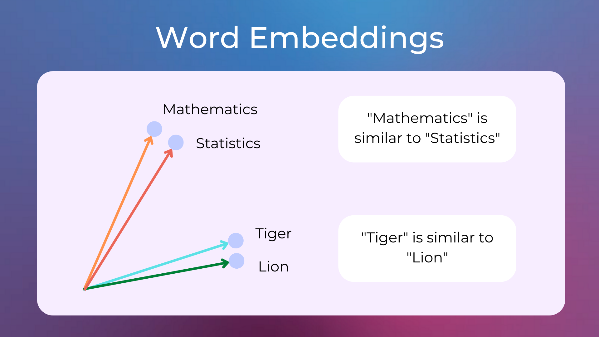
Fig 1. Scheme of a 2-D representation of the words "statistics", "mathematics", "Tiger" and "Lion". Source: https://www.nlplanet.org/course-practical-nlp/01-intro-to-nlp/11-text-as-vectors-embeddings

For this post we only need to know that we can use the embeddings that LLMs use for other things than making queries (prompting) to a LLM.

In this short demonstration we are going to use language models -that were developed to analyze sentences (sentence-transformers)- to find articles on Arxiv that might be useful for a particular project, using keywords and a description of the project (or abstract) we want to develop.

For simplicity and to reduce computational time, we are going to divide the search process into the following steps:

• Step 1: Filter the articles that cointain specific or general keywords that we want to look for

• Step 2: Compute similarities between the abstracts from the papers that we collected and the article of reference

• Step 3: Sort collected articles by similarity values

This way we don't need to calculate similarities from articles that don't include our keywords, and we can expect to find useful some of the articles from the top of the list.

Let's start with importing the libraries we are going to use:

# import libraries

#for numerical calculations
import numpy as np

# for files and directories
import os
import json

# plotting
import matplotlib.pyplot as plt
#%matplotlib inline

#regex
import re

and to retrieve ArXiV's information we can download their MetaData Dataset from Kaggle. This dataset provides the following information for every article on ArXiV:

• id: ArXiv ID (can be used to access the paper)

• submitter: Who submitted the paper

• authors: Authors of the paper

• title: Title of the paper

• comments: Additional info, such as number of pages and figures

• journal-ref: Information about the journal the paper was published in

• doi: https://www.doi.org

• abstract: The abstract of the paper

• categories: Categories / tags in the ArXiv system

• versions: A version history

once we have downloaded the dataset, we can either load it or stream it. Since the dataset is aroud ~ 4GB, instead of loading the file we are going to use the yield keyword to iterate over the lines without storing the entire file in memory:

# Arxiv metadata dataset ~ 1.7 million of papers

# File address
data_file = "~\arxiv-metadata-oai-snapshot.json"

""" get_metadata(data_file)

    Function to get metadata from the json file
    Args: data_file: name of the file (with full path if needed)  
    Returns: yields the lines from the json file

"""
def get_metadata(data_file):
    with open(data_file, 'r') as f:
        for line in f:
            yield line

Now we can test our function get_metadata() to print out the data for the first paper

# get the metadata
arxiv_metadata = get_metadata(data_file)

# Printing the values of the first paper in the dataset by breaking the loop after the first iteration
for paper in arxiv_metadata:
  for k, v in json.loads(paper).items():
    print(f'{k}: {v}')
  break

id: 0704.0001
submitter: Pavel Nadolsky
authors: C. Bal\'azs, E. L. Berger, P. M. Nadolsky, C.-P. Yuan
title: Calculation of prompt diphoton production cross sections at Tevatron and
  LHC energies
comments: 37 pages, 15 figures; published version
journal-ref: Phys.Rev.D76:013009,2007
doi: 10.1103/PhysRevD.76.013009
report-no: ANL-HEP-PR-07-12
categories: hep-ph
license: None
abstract:   A fully differential calculation in perturbative quantum chromodynamics is
presented for the production of massive photon pairs at hadron colliders. All
next-to-leading order perturbative contributions from quark-antiquark,
gluon-(anti)quark, and gluon-gluon subprocesses are included, as well as
all-orders resummation of initial-state gluon radiation valid at
next-to-next-to-leading logarithmic accuracy. The region of phase space is
specified in which the calculation is most reliable. Good agreement is
demonstrated with data from the Fermilab Tevatron, and predictions are made for
more detailed tests with CDF and DO data. Predictions are shown for
distributions of diphoton pairs produced at the energy of the Large Hadron
Collider (LHC). Distributions of the diphoton pairs from the decay of a Higgs
boson are contrasted with those produced from QCD processes at the LHC, showing
that enhanced sensitivity to the signal can be obtained with judicious
selection of events.

It seems that our code is working so far. Now, lets take as case of study a paper already published in a journal that contains keywords and abstract.

Because I find collective behavior fascinating, and I have always wanted to work on a project that studies collective behaviour in football (yes, the real one). Let's try to find papers that approach the study of collective behaviour in football in the way researchers study animal systems.

We are going to use this really cool paper: Searching for structure in collective systems by Twomey et al. where they develop a methodology to quantify coordination and identify the most (and least) coordinated components in multi-individual systems.

Now, in order to start our search, lets define some of the variables we are going to use. For this particular case I want to find papers that study football, so I will make that keyword a must for my search, and I will define some secondary keywords that will help us to find more papers.

#the main keywords
keywords_all = ['soccer'] # Soccer... :facepalm:

#secondary keywords
keywords_any = ['collective','behaviour','behavior','human','sports', 'football']

#the abstract/description we are going to use as reference
abstract_reference = ['From fish schools and bird flocks to biofilms and neural networks, collective systems in nature are made up of many mutually influencing individuals that interact locally to produce large-scale coordinated behavior. Although coordination is central to what it means to behave collectively, measures of large-scale coordination in these systems are ad hoc and system specific. The lack of a common quantitative scale makes broad cross-system comparisons difficult. Here we identify a systemindependent measure of coordination based on an information-theoretic measure of multivariate dependence and show it can be used in practice to give a new view of even classic, well-studied collective systems. Moreover, we use this measure to derive a novel method for finding the most coordinated components within a system and demonstrate how this can be used in practice to reveal intrasystem organizational structure.']

To search for the keywords we can define some functions

""" contains_any(keywords, text)

    Function that recevies a list of keywords and a text and returns True if any of the keywords is in the text
    input: keywords, text: as strings.
    returns: True if any of the keywords is in the text, False otherwise.
"""
def contains_any(keywords, text):
    pattern = r"\b(" + "|".join(keywords) + r")\b"
    return bool(re.search(pattern, text, flags=re.IGNORECASE))

""" contains_all(keywords, text)
    
    Function that recevies a list of keywords and a text and returns True if all of the keywords are in the text
    input: keywords, text: as strings.
    returns: True if all of the keywords are in the text, False otherwise.    
    
"""
def contains_all(keywords, text):
    return all(word in text for word in keywords)

Now we can start searching and collecting the MetaData from the papers that include "soccer" and/or the secondary keywords in their title or abstract

num_papers = 500 #setting a limit for retrieved papers, just in case we get too many
counter_ = 0    #counter for the number of papers retrieved
collected_papers = []
#getting the metadata
arxiv_metadata = get_metadata(data_file)

#iterating over the metadata
for paper in arxiv_metadata:
    #loading the information of the paper
    paper_info = json.loads(paper)
    #checking if the paper contains the primary keywords
    if contains_all(keywords_all, paper_info['abstract'].lower()) or contains_all(keywords_all, paper_info['title'].lower()):
        #secondary keywords
        if contains_any(keywords_any, paper_info['abstract'].lower()) or contains_any(keywords_any, paper_info['title'].lower()):
            #we collect the paper
            collected_papers.append(paper_info)
            counter_ += 1
    #if we have reached the limit we break the loop
    if counter_ == num_papers:
        break

print(f"Total papers collected: {len(collected_papers)}")

Total papers collected: 227

It seems that we didn't need to break the loop since we only found 227. If we want to retrieve more papers we could modify our keywords (adding more to the secondary keywords array), but we don't need that for this example.

Let's print out the first 10 articles that we found

[print(collected_papers[i]['title'] + '\n') for i in range(15)]

Movement and Man at the end of the Random Walks

New Mechanics of Generic Musculo-Skeletal Injury

Using the Sound Card as a Timer

Dynamics of tournaments: the soccer case

Relative Age Effect in Elite Sports: Methodological Bias or Real
  Discrimination?

Soccer: is scoring goals a predictable Poissonian process?

The Socceral Force

Relative locality and the soccer ball problem

Archetypal Athletes

Learning RoboCup-Keepaway with Kernels

Towards Real-Time Summarization of Scheduled Events from Twitter Streams

A statistical view on team handball results: home advantage, team
  fitness and prediction of match outcomes

How does the past of a soccer match influence its future?

Quantum Consciousness Soccer Simulator

Inferring Team Strengths Using a Discrete Markov Random Field

With a little inspection we can notice that the articles seem to be related to soccer and even if they might contain some of our keywords, it is not very clear how many (if any) of them are going to be helpful for us. In order to retrieve the most helpful articles for our study, we can now compute how similar their abstracts are with respect to our abstract of reference.

First we import the libraries we are going to use for the embeddings

# Importing the necessary libraries for llms
from transformers import *
from sentence_transformers import SentenceTransformer, util

The embedding we are going to use is from the model paraphrase-MiniLM-L6-v2 and details about it can be found here. This model was trained particularly to derive semantically meaningful sentence embeddings and compare them using cosine similarity. If you want to know about how the model was developed you can check the ArXiV paper here or check the documentation for more details about the package sentence_transformers.

Now let's load and inspect the model

# We are going to use one of the models from the sentence-transformers library to get the embeddings of the sentences
model_name = 'paraphrase-MiniLM-L6-v2'
llm_model = SentenceTransformer(model_name)

loading configuration file config.json from cache at C:\Users\.cache\huggingface\hub\models--sentence-transformers--paraphrase-MiniLM-L6-v2\snapshots\3bf4ae7445aa77c8daaef06518dd78baffff53c9\config.json
Model config BertConfig {
  "_name_or_path": "sentence-transformers/paraphrase-MiniLM-L6-v2",
  "architectures": [
    "BertModel"
  ],
  "attention_probs_dropout_prob": 0.1,
  "classifier_dropout": null,
  "gradient_checkpointing": false,
  "hidden_act": "gelu",
  "hidden_dropout_prob": 0.1,
  "hidden_size": 384,
  "initializer_range": 0.02,
  "intermediate_size": 1536,
  "layer_norm_eps": 1e-12,
  "max_position_embeddings": 512,
  "model_type": "bert",
  "num_attention_heads": 12,
  "num_hidden_layers": 6,
  "pad_token_id": 0,
  "position_embedding_type": "absolute",
  "transformers_version": "4.39.2",
  "type_vocab_size": 2,
  "use_cache": true,
  "vocab_size": 30522
...
}

One of the first thing we notice is that this model is based on BERT and that the embedding that it uses has 384 dimensions (hidden size). To corroborate that, we can encode (pass through the model a sentence and get its emmbeding) the abstract we are going to use for reference:

# Getting the embeddings of the reference abstract
abstract_em = llm_model.encode(abstract_reference)
# Printing the shape of the embeddings
print(np.shape(abstract_em))

(1, 384)

Now, with this numerical representation of our abstract in the 384-dimensional space of this model, we can quantify how semantically close the abstracts (papers retrieved) are to our reference.

#storing values
sim_values = []
collected_titles = []
collected_abstracts = []
collected_arxiv_ids = []
collected_doi = []

#iterating over the collected papers
for paper in collected_papers:
    #storing each of the important values we want to keep
    collected_titles.append(paper['title'])
    collected_abstracts.append(paper['abstract'])
    collected_arxiv_ids.append(paper['id'])
    collected_doi.append(paper['doi']) 
    #finally computing the similarity between abstracts and store it
    sim_values.append(float(util.cos_sim(abstract_em, llm_model.encode(paper['abstract']))[0][0].detach().numpy()))

And we can do a quick inspection of the first 15 papers

# print the titles oredered by s with the reference title.
np.array(collected_titles)[np.argsort(sim_values)][::-1][0:14]

array(["Stochastic model for football's collective dynamics",
       'Using network science to analyze football passing networks: dynamics,\n  space, time and the multilayer nature of the game',
       'A Continuous-Time Stochastic Process for High-Resolution Network Data in\n  Sports',
       'The Soccer Game, bit by bit: An information-theoretic analysis',
       'Modeling ball possession dynamics in the game of football',
       'A new method for comparing rankings through complex networks: Model and\n  analysis of competitiveness of major European soccer leagues',
       'Emergent Coordination Through Competition',
       'Deep Decision Trees for Discriminative Dictionary Learning with\n  Adversarial Multi-Agent Trajectories',
       'Optimising Long-Term Outcomes using Real-World Fluent Objectives: An\n  Application to Football',
       'Hierarchical and State-based Architectures for Robot Behavior Planning\n  and Control',
       'Primacy & Ranking of UEFA Soccer Teams from Biasing Organizing Rules',
       "Disruptive innovations in RoboCup 2D Soccer Simulation League: from\n  Cyberoos'98 to Gliders2016",
       'Alterations in Structural Correlation Networks with Prior Concussion in\n  Collision-Sport Athletes',
       'Optimising Game Tactics for Football'], dtype='<U145')

Just by looking at the first five papers, I can confirm that I do recognize some of them because this is a topic I am very interested in. But this search already added a lot of references I wasn't aware of, so I'm excited to read them as well!

Finally, we can save the papers we found in a DataFrame and export it as .csv

import pandas as pd
# indexing the papers by the similarity value in decreasing order
ix_order = np.argsort(sim_values)[::-1]
# Creating a pandas DataFrame with the collected data
df = pd.DataFrame({'title': np.array(collected_titles)[ix_order], 
                   'abstract': np.array(collected_abstracts)[ix_order], 
                   'arxiv_id': np.array(collected_arxiv_ids)[ix_order], 
                   'doi': np.array(collected_doi)[ix_order], 
                   'similarity': np.array(sim_values)[ix_order]})

# saving the dataframe as csv
df.to_csv('collective_football_biblio.csv', index=False)

Here you can find the notebook for this post.